Final Report Kinematic and Structural Design Optimization of a Small-Scale Formula-Style

Anthony Klepacki

Advisor: Professor James Allison

Abstract

Formula SAE is an on-campus engineering RSO that designs and builds a small-scale, formula-style racecar where a lightweight and objective-driven suspension is critical in achieving desired performance at competition. Designing a lightweight suspension with desired characteristics such as low bump steer and a tire-specified camber gain rate becomes a non-trivial engineering design problem due to the geometrical non-linearities, as well as coupling between elastic deformation and changes in the ultimate suspension characteristics. A SQP based optimization solver is used along with a custom-developed elasto-kinematic and structural suspension solve in order to design a new double a-arm independent pushrod suspension for the Illini Motorsports SAE formula racecar. A desired $0^{\circ}\ deg/inch$ bump-steer rate and $2^{\circ}\ deg/inch$ camber gain rate is set as the objective, while continuously minimizing mass on each of the six independent suspension links. The starting seed point for the optimizer is the 2016-2017 rear suspension of the Illini Motorsports SAE racecar, but a multi-start strategy is also implemented to avoid the potential of local minima. Ultimately, a suspension that is able to achieve a desired $0^{\circ}\ deg/inch$ bump-steer rate and $2^{\circ}\ deg/inch$ camber gain rate while having a 14% reduction in overall mass.

Introduction

2.1 – Problem Scope and Literature Review

Formula SAE is an on-campus engineering RSO that designs and builds a small-scale, formula-style racecar, and subsequently participates in international competitions every year [1]. One of the main major focuses of each competition entry racecar is the design and manufacturing of the vehicle suspension which attempts to maximize the capacity of grip produced by the tires and transfer those loads effectively and efficiently to the chassis and ultimate to the rest of the vehicle. The suspension is a critical subsystem assembly that must be properly designed around the rest of the specific vehicle architecture and thus results in a application specific setup with a vast number of configurations.

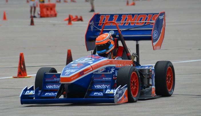
Figure 1 - Illini Motorsports Formula SAE Racecar [9]

This typically takes the form of a coupled, multi-variable non-linear design problem, where an intensive understanding of kinematics is required to develop intuition to understand how changes to the system architecture effect the overall response of the vehicle. Milliken et al. [3] provide general guidelines in using geometric axis projection methods as simple design techniques to create a baseline suspension. This allows the design to target generalized camber and bump-steer curves, but Milliken also states that the coupled nature of independently design the suspension about each axis leads to unforeseen kinematics which can only be adjusted through on-track testing or through high expensive instrumented prototypes. The design is typically iterated through in a trial and error fashion, with analysis provided through various kinematic solvers. This becomes a very cumbersome and time-consuming design process to find ideal characteristics while maintaining desired solutions, and thus a coupled multi-objective optimization solver with elasto-kinematics can reduce the cost at the front end of design to delve deeper into a more functional baseline suspension design.

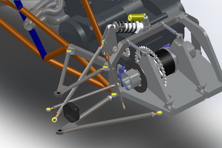
Figure 2 - Typical FSAE Suspension Setup in context

A double independent a-arm suspension enables the suspension to have a movement arc of the second order, as compared to for instance a McPherson strut suspension which is limited to a first order (circular) curve [3]. This allows for a high degree of design flexibility since a better approximation to a linear camber gain can be design for, but this adds a degree of complexity in targeting such an objective. Thus, an elasto-kinematic framework and optimization solver would be to design a suspension with the intent of setting desired characteristics and having the solver find the ideal distribution of points that achieve the desired kinematic response, as opposed to the conventional form, which would select points first and then find response. This would include setting performance targets for kinematic suspension characteristics such as [3,4]:

Camber gain
Toe response
Bump steer

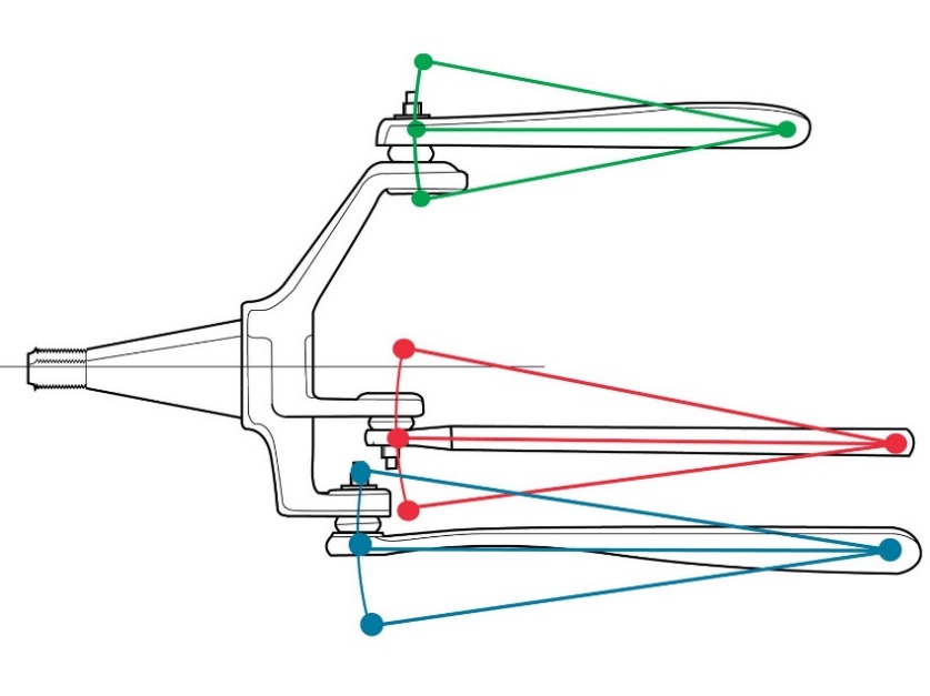
Figure 3 - Double A-arm movement [3]

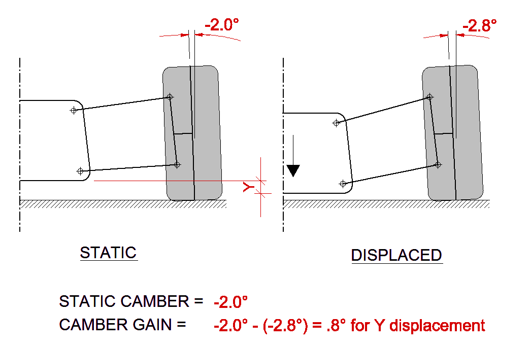
Figure 4 - Example of desired kinematic response; Camber Gain [8]

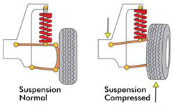
Figure 5 - Example of desired kinematic response; Bump Steer [7]

2.2 - Problem Formulation

The optimization problem of the coupled kinematic and structural suspension solver takes the general form of an optimization problem as the following:

$\operatorname{}{\ \{ f_{1}\left( \mathbf{x} \right),f_{2}\left( \mathbf{x} \right),\ldots,f_{n}\left( \mathbf{x} \right)\}}$ $\text{subject\ to\ }\left\{ g_{1}\left( \mathbf{x} \right),g_{2}\left( \mathbf{x} \right),\ldots,g_{m}\left( \mathbf{x} \right) \right\} \leq 0$

Where there are many objective functions which dictate the kinematic response of interest, as well as the structural integrity of the system. The following are examples of the objective functions, but can be extended to various other kinematic response criterion [3,4,5]:

$f_{1}\left( \mathbf{x} \right) \equiv total\ system\ mass$ $f_{2}\left( \mathbf{x} \right) \equiv bump\ steer\ repsonse - L_{2}\text{Norm\ minimization\ between\ objective\ and\ result}$ $f_{3}\left( \mathbf{x} \right) \equiv camber\ gain\ repsonse - L_{2}\text{Norm\ minimization\ between\ objective\ and\ result}$

The constraints take the form of structural sizing constraints, as well as deformation and manufacturing constraints [2]

$g_{1}\left( \mathbf{x} \right) \equiv material\ yield\ in\ suspension\ links$ $g_{2}\left( \mathbf{x} \right) \equiv material\ instability\ and\ buckling\ limit\ loads$ $g_{3}\left( \mathbf{x} \right) \equiv maximum\ and\ minumum\ manufacturable\ lengths$ $g_{4}\left( \mathbf{x} \right) \equiv \ maximum\ and\ minumum\ manufacturable\ tube\ sizes$

The problem formulation is calculated to a set of design variables which are the lengths of each of the six links that make up the suspension

$\mathbf{x} = \{ Upper\ a - arm\ Front\ Length;\ Upper\ a - arm\ Rear\ Length;Lower\ a - arm\ Front\ Length;\ Lower\ a - arm\ Rear\ Length;Toe\ link,\ Push - rod\ Length\}$

System Model and Model Analysis

3.1 - Kinematic Modelling – Rigid Body Motion

The primary result of the solver for the optimization problem will be based on a simple elasto-kinematic solver for the suspension motion through the anticipated range of motion. The suspension of interest is a double independent a-arm suspension and thus it can be modelled as a six-bar linkage, as can be seen in the following image [3,4].

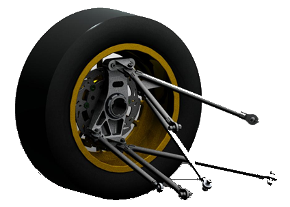
Figure 6 - Typical A-arm suspension

To model the motion the theory of rigid body kinematic will be used, with the inputs being the lengths of each of the links (this is also the set of design variables in the optimization problem). The points that define the inboard chassis-side points of the suspension are kept as constant since these are typically set at the beginning of the design process. Using a set of constraint equations which are defined by solving for the set of outboard points by solving a system of equations that constraints the distance between each of the points, the resulting points are the outputs of the model. By varying the ride-height, which is a function of length of the push-rod, the full range of motion can be solved for. Once this temporal distribution and motion of the points is modelled, a set of kinematic response can be calculated from using the relative geometries of the suspension with regards to the global coordinates system (camber, toe, bump steer, etc.) [5].

$Rigid\ Body\ Kinematics \equiv f(\left\{ link\ length;inboard\ points \right\} = outboard\ points\$

The constrain equations are based on calculating the distances between each of the points connected by the links and using a non-linear equation solver (such as the ‘fsolve’ solver in Matlab) to find the associated outboard that connect the assumed inboard points by the design point link lengths. The data structure for the array of points are as follows:

$points = \{ LCA_{\text{front}},LCA_{\text{rear}},LCA_{\text{outboard}},UCA_{\text{front}},UCA_{\text{rear}},UCA_{\text{outboard}},Tierod_{\text{inner}},$ $\text{Tiero}d_{\text{outer}},Pushrod_{\text{inner}},Pushrod_{\text{outer}}\}'\ \$

Where each of the points is a three-dimensional spatial representation of cartesian coordinates associated with the points, such as in the example of the lower control arm front points:

$\text{LC}A_{\text{front}} = \{ LCA_{front,x},LCA_{front,y},LCA_{front,z}\}$

The distances between points of two associated points is computed as the Euclidean vector norm, such as in the example as the length between the lower control arm front and lower control arm outboard points:

$Distance = D\left( v_{1},v_{2} \right) = \sqrt{\sum\left( v_{1i} - v_{2i} \right)^{2}}\ for\ i = \left\{ 1,2,3 \right\}$ $\text{Lengt}h_{LCA,front} = D\left( \text{LC}A_{\text{front}},\text{LC}A_{\text{outboard}} \right)$ $\text{Lengt}h_{LCA,front} = \sqrt{\left( \text{LC}A_{front,x} - LCA_{outboard,x} \right)^{2} + \left( \text{LC}A_{front,y} - LCA_{outboard,y} \right)^{2} + \left( \text{LC}A_{front,z} - LCA_{outboard,z} \right)^{2}}$

The full system of equations is then setup for each of the link lengths of the control arms (6 equations), as well as an extra system of equations that constrains the tierod (3 equations) and the connection point of the pushrod in the plane of the lower control arm (3 equations) resulting in a system of 12 total equations which are then used to solve for the each of the 3 components of the 4 outboard suspension points of interest (12 unknowns), which results in a full kinematically constrained and solvable system.

Lower Control Arm Constraint Functions

$D\left( \text{LC}A_{\text{front}},\text{LC}A_{\text{outboard}} \right) - Length_{LCA,Front} = 0$
$D\left( \text{LC}A_{\text{rear}},\text{LC}A_{\text{outboard}} \right) - Length_{LCA,rear} = 0$

Upper Control Arm Constrain Functions

$D\left( \text{UC}A_{\text{front}},\text{UC}A_{\text{outboard}} \right) - Length_{UCA,Front} = 0$
$D\left( \text{UC}A_{\text{rear}},\text{UC}A_{\text{outboard}} \right) - Length_{UCA,rear} = 0$

Upright Height Constrain Function

$$D\left( \text{UC}A_{\text{outboard}},\text{LC}A_{\text{outboard}} \right)
- 9.3948 = 0$$
$D\left( \text{Pushro}d_{\text{inner}},Pushrod_{\text{outer}} \right) = Length_{\text{pushrod}} = 0$

Tierod Constrain Function

$$D\left( \text{Tiero}d_{\text{inner}},\text{Tiero}d_{\text{outer}} \right)
- Length_{\text{tierod}} = 0$$
$D\left( \text{Tiero}d_{\text{outer}},LCA_{\text{outer}} \right) - 3.0134 = 0$
$D\left( \text{Tiero}d_{\text{outer}},UCA_{\text{outer}} \right) - 8.9621 = 0$

Lower Control Arm Pushrod Interface Constrain Functions (Distance taken from master CAD Model)

$D\left( \text{LC}A_{\text{front}},Pushrod_{\text{outer}} \right) - 15.5987 = 0$
$D\left( \text{LC}A_{\text{rear}},Pushrod_{\text{outer}} \right) - 1.8485 = 0$
$D\left( \text{Pushro}d_{\text{inner}},Pushrod_{\text{outer}} \right) - RideHeight = 0$

$Function\ Set\ for\ fsolve \equiv f_{\text{set}} = \begin{Bmatrix} Eq\ 1 \\ \vdots \\ Eq\ 12 \\ \end{Bmatrix}$ $\text{fsolve}\left( f_{\text{set}} \right) = Outboard\ Points$ $Outboard\ Points \equiv \left\{ P \right\} = \begin{Bmatrix} \begin{matrix} \{ LCA_{\text{outer}}\} \\ \{ UCA_{\text{outer}}\} \\ \end{matrix} \\ \begin{matrix} \{ Tierod_{\text{outer}}\} \\ \{ Pushrod_{\text{outer}}\} \\ \end{matrix} \\ \end{Bmatrix}$

The primary vertical motion of the suspension which enables the assembly to kinematically move in jounce and rebound is the relative length or motion of the pushrod. For simplicity a pseudo ride-height movement is implemented by approximation the range of motion as the distance that the pushrod can contract and expanding, which is analogous to the spring-damper system on an actual racecar compressing and expanding. This is then used to solve the distribution of points at each ride-height step thus giving a pseudo-temporal movement of the suspension through its range of motion.

$Nominal\ Ride\ Height \equiv D$ $Motion\ Range \equiv D - x \leq D \leq D + x\ where\ x = \frac{(range\ max - range\ min)}{\text{motion\ steps}}$

Finally, this data is passed through the elasto-kinematic sub-function (see section: Structural Solving below) and the objective functions are ultimately computed. The mass objective function is simple to calculate by the following relation:

$Total\ system\ mass \equiv m = \sum\rho_{\text{material}}A_{cross - section,i}*L_{i}\ for\ i \in \{ links\}$

The two kinematic curves of interest, namely the camber gain and bump steer are computed by geometrical projection of the relevant suspension links of interest onto their respective spatial planes. For camber gain this is the projection of vector between the upper and lower control a-arm outboard points onto the [1,0,0]’ plane, and for bump steer this is the projection of the vector the upper and lower control a-arm outboard points onto the [0,0,1]’ plane, all of which is defined in the standard SAE J670 coordinate system [10]. This is calculated at each pseudo-temporal motion step to produce a curve of camber and bump steer through the ride-height (shown below) and this is later decomposed to computer the final objective functions.

The final representation of the suspension can also be visualized in an animated and rendered format for visual inspection of the baseline solution to check for errors:

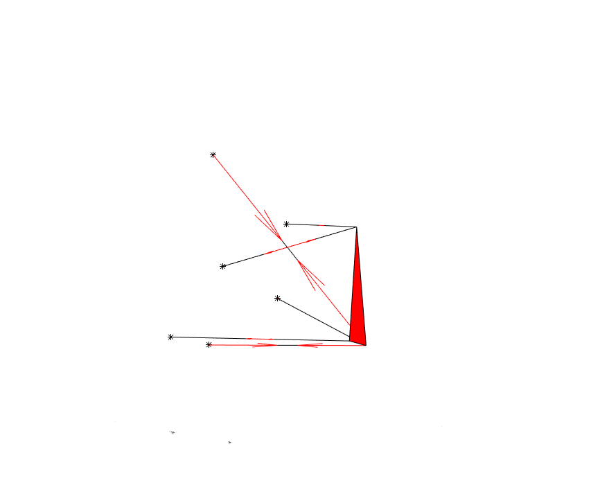
Figure 7 - MATLAB Solver (by Anthony Klepacki) showing kinematic motion, as well as relative forces under loading

3.2 - Structural Solving

Finding the suspension forces is a basic statics problem. A corner assembly is composed of 6 links (front and rear upper/lower a-arms, toe/steering links, and push/pull rods), each interfacing with an upright, as well as to the chassis. This gives us 6 two force members. Modelling these are two-force member gives a system of 6 unknowns for the tension/compression forces through each of these links. To solve this system, it is necessary to find six equations to create a complete system which can be solved. This is solved through a force and moment balance in three dimensions. The equations below outline the general solution for simultaneously solving the complete system of 6 unknowns with their corresponding six equations [2].

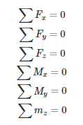
Force acting on upright (below). These forces need to be counteracted by the external forces from the contact patch. This is solved using a static force and moment balance where the sum of all the forces and the sum of all the moments, in all three dimensions (x, y and z), need to sum to zero. In order words, the forces and resultant moments produced by each of the six-suspension links must sum to the external forces and moments acting on the upright from the contact patch [6].

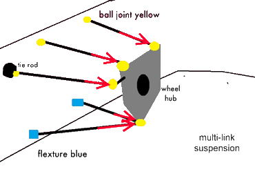
Figure 8 - Structural Sizing based on six bar linkage equations

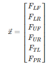
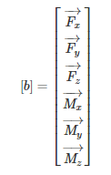
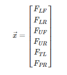
The above solution is then used to back calculated the strains in each of the suspension links by the simple solid mechanics relations that dictate deformation on a cylindrical tube, and the material parameters [2].

$\sigma = \frac{\text{Force}}{\text{Area}}$ $\epsilon = \frac{\sigma}{E}$ $L = \left( 1 + \epsilon \right)L_{0}$

Once the change in deformation is applied, another round of the kinematic solver is simulated to have an approximate elasto-kinematic response. The optimization problem then works to solve the kinematic response curves of interest (i.e. bump steer, camber gain, etc.) in a least square fit, along with minizine the total system mass). The mass is dictated by the structural sizing, which is material dependent and involves two main failure modes, yield and buckling, which is defined as follows [2]:

$\sigma_{\text{yield}}\left( \text{Material} \right) \geq \ \sigma_{\text{applied}} = \frac{\text{Force}}{\text{Area}}$ $F_{\text{buckling}}(Tube\ Thickness,\ Material\ Allowables,\ Length,\ Geometry) \geq F_{\text{applied}}$ $F_{buckling,Euler} = c\frac{\text{πEI}}{L^{2}}$

The forces at the contact patch are calculated for three load cases which are derived from doing vehicle dynamics simulations based on the 2017 competition entry vehicle. The first load case is the case for maximum lateral loading (max cornering), the second is maximum longitudinal loading (max braking/deceleration), and the final one is a combined case which takes the maximum force components of each of the prior two cases and envelopes them.

$Force\ Set \equiv F_{\text{set}} = \begin{Bmatrix} F_{x} \\ F_{y} \\ F_{z} \\ \end{Bmatrix}$

The maximum cornering forces enveloped across the four corners of the car are:

$F_{set,cornering} = \begin{Bmatrix} 0 \\ 551.95 \\ - 412.83 \\ \end{Bmatrix}\text{lbf}$

The maximum braking forces enveloped across the four corners of the car are:

$F_{set,cornering} = \begin{Bmatrix} 521.16 \\ 0 \\ - 383.1 \\ \end{Bmatrix}\text{lbf}$

The maximum combined (cornering and braking) forces enveloped across the four corners of the car are:

$F_{set,cornering} = \begin{Bmatrix} 521.16 \\ 551.95 \\ - 412.83 \\ \end{Bmatrix}\text{lbf}$

The solver computes the maximum resultant force in each of the links independently from the enveloped link forces across the three load cases. These results are then supplied for the yield sizing, where the criterion takes the value in tension as the limit load, and for buckling sizing, where the criterion takes the load in compression as the limit load. Both constraints are simultaneously optimized for with a supplied factor of safety against the specified material allowables before looping through the elasto-kinematic solver until the total system mass tolerance is met.

3.3 - Solution Roadmap

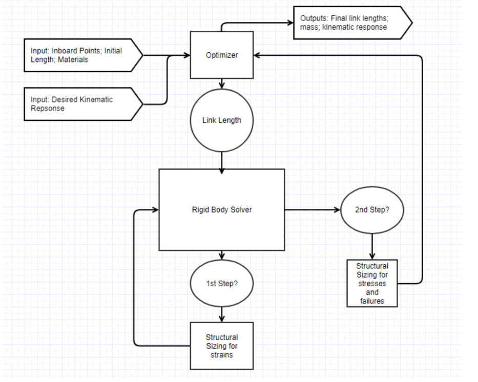
A visual representation of the elasto-kinematic solver is shown below as a simplified roadmap of each of the solution stages and passage of data throughout the solver:

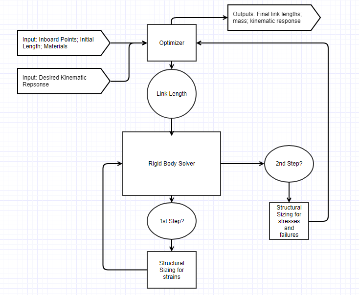
Figure 9 - Simplified Flowchart Representation of Suspension Solver

3.4 - Assumptions and Uncertainty Analysis

This kinematic solver is based on a primarily rigid body solver with a very simple implementation of elasto-kinematics. The elasto-kinematic solver uses an iterative method, rather than a full-simultaneous solver to compute the strains at which each of the links deform. A simple parametric study was preformed to see the necessity of the iterative elasto-kinematic solver in two configurations. The first configuration is the sizing of the links per the current Illini Motorsports suspension structural sizing design, which was designed using a conventional solid mechanic approach for yield and bucking. The second was using the structural sizing optimizer implemented within the solver which calculates the lowest mass inner and outer diameter for each of the links. For the first configuration the elasto-kinematic solver only calculated a single iteration showing the strain was below the tolerance of the solver and thus not enough to affect the kinematic solution. In the second configuration an average of three iterations were required to reach a steady state mass calculation, showing that at optimal sizing the strains are much higher than currently seen. Since this is a very non-linear and coupled result to the final kinematics of the structure a sensitivity study will be performed in the future to investigate the effects of cross sectional area of each of the links to the resulting strains and assembly kinematics.

A second assumption of the overall problem formulation is that the inboard points of the suspension are assumed to be fixed. This is typically dictated largely by chassis architecture on a motorsports vehicle and is beyond the scope of the current project framework. Nonetheless, as sensitivity study will be performed to see the relative effects of moving inboard points compared to moving outboard points and the computational cost required to reach the objective functions.

Finally, a parametric study will be done for the rigid body kinematic effects of moving each of the points in each of the three primary axes individually. This will be performed to develop a baseline intuition on the effects of independent changes in suspension points and the track down which of the points become coupled to attempt to simplify the problem formulation.

The preliminary list of parametric and sensitivity studies to be performed will be:

Structural Sizing sensitivity
Inboard points parametric study
Movement of outboard points parametric study

Optimization Studies and Results

4.1 - Parametric studies

A series of parametric studies is performed to find the sensitivity of each of the suspension characteristics of interest with respect to a perturbation of a discrete point of the suspension. Each of the points is perturbed by 0.05 inches, which is the typical manufacturing tolerance of the Formula SAE racecar, in both direction and in all three spatial degrees of freedom (+/-X, +/-Y, and +/-Z). The results are plotted on equivalent axes in order to gauge the relative sensitivities of each of the plots.

- Parametric Study of the camber gain performance of a push-rod suspension

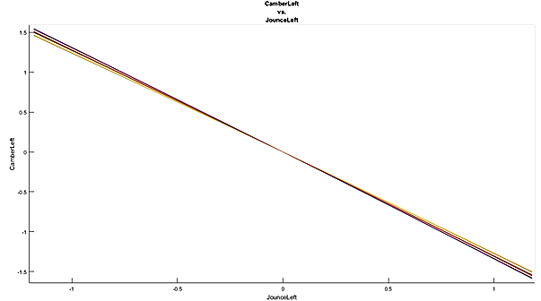
Figure 10 - Relative Sensitivities of camber gain vs. perturbation of suspension points

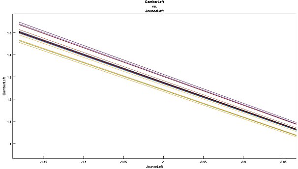
Figure 11 - Detailed section of end of range of motion showing clustering of sensitivities

Table 1 - Tabulated statistics of camber gain parametric study

	Sensitivity Spread Statistics
	Negative Jounce Max	Neutral Jounce	Positive Jounce Max
Average	0.50006	1.38E-12	-0.51485
St. Dev	0.70917	1.96E-12	0.72927

From the two plots above it can be seen that there is a strong clustering of certain suspension points having a greater impact into the resulting camber gain of the perturbed suspension. These points correlate with the lower and upper a-arm points. This follows intuition since these points are typically decided in pseudo-closed form solutions to calculate a rough overall camber gain. These solutions do not take into account the non-linearity of the camber gain curve throughout the +/- 1-inch jounce of the suspension, as can be seen in the parametric study curves. This study will be used as a spot check for the finite difference gradients calculated by the optimizer in the following section. The final observation is that there is a lack of symmetry in the solution of the parametric study. In other words, this means that there is a larger sensitivity in the positive jounce direction as compared to the negative jounce direction. This is due to the unequal a-arm lengths that are typically implemented in a motorsports type of suspension, with the upper set of a-arm’s being longer than the lower set.

4.1.2 - Parametric Study of the camber gain performance of a push-rod suspension

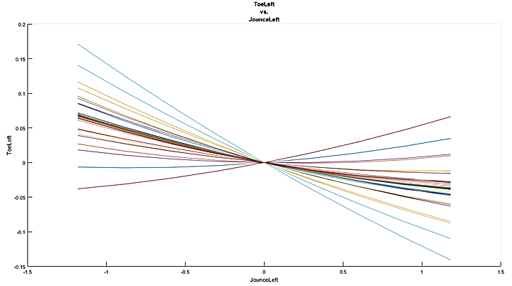
Figure 12 - Relative Sensitivities of bump steer vs. perturbation of suspension points

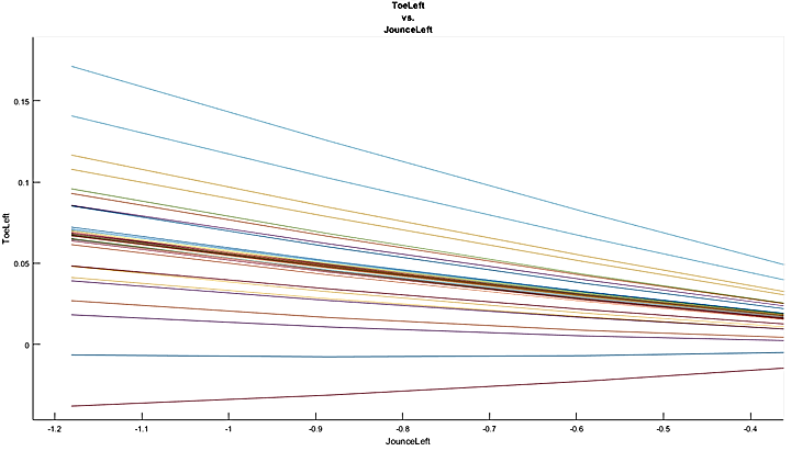
Figure 13 - Detailed section of end of range of motion showing clustering of sensitivities

Table 2 - Tabulated statistics of bump steer parametric study

	Sensitivity Spread Statistics
	Negative Jounce Max	Neutral Jounce	Positive Jounce Max
Average	0.022421	8.80E-12	-0.012483
St. Dev	0.0339	6.21E-12	0.02133

The second parametric study is done on the bump steer sensitivity. This is performed in the same perturbation manner as the camber gain parametric study. From the plots we can see that even though there is a lower absolute sensitivity in the bump steer due to the already low amount of bump steer on the 2016-2017 rear pushrod suspension, there is a large relative sensitivity of bump steer for certain points. For instance, the largest sensitivity is for the outer tie-rod points, and this captures the entire range of the sensitivities. This means that a perturbation of this point can not only drastically change the value of the resulting bump steer, but it can also change the sign of the bump steer curve, thus rending it unstable. This can potentially lead to problems in convergence of the optimization solver since this can lead to a more ill-posed problem formulation. Finally, we observe again that there is lack of symmetry with a larger sensitivity to bump steer in the negative jounce direction, as opposed to a larger sensitivity in the positive jounce direction for camber gain.

Optimization Problem 1 – Optimized Camber Gain

The optimization results of the elasto-kinematic solver with structural sizing optimization are outlined below. The points for the baseline 2017 Illini Motorsports suspension are chosen as the starting solution, and these are exported from the master computer aided design (CAD) model as a point cloud (rigid upright shown in red; links shown in black).

Solution Initialization Points.
$\text{LC}A_{\text{front}} = \$ [39.0586;-9.42;5.735];
$\text{LC}A_{\text{rear}}\$ =[27.7246;-9.42;6.126];
$\text{LC}A_{\text{outboard}}\$ =[38.1866;-22.961;5.425];
$\text{UC}A_{\text{front}}\$ = [39.0976;-10.624;12.406];
$\text{UC}A_{\text{rear}}$ = [28.4506;-10.624;12.668];
$\text{UC}A_{\text{outboard}}$ = [37.2096;-22.11;14.73];
$\text{Pushro}d_{\text{inner\ }}$ =[37.5996;-9.022;20.861];
$\text{Pushro}d_{\text{outer}}\$ = [37.3996;-21.651;6.465];
$\text{Tiero}d_{\text{inner}}\$ = [40.9476;-7.047244095;6.5807];
$\text{Tiero}d_{\text{outer}}$ = [40.9476;-22.987;6.632];

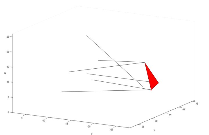
Figure 14 - Baseline Illini Motorsports 2017 Suspension Setup (links: black; Upright; red)

Problem Initialization and Constants

For the optimization algorithm a sequential quadratic problem (SQP) algorithm is chosen with line-search. The tolerances are chosen to be default since the 1e-6 tolerance of the objective and constraint functions captures the realistic limitations of the material characteristics as well as the manufacturing limits that can be realistically made. The links lengths are then computed using the distance function (see section: Rigid Body Kinematics) and the problem is initialization with the following parameters

Motion Simulation Parameters:
- +1/-1 inch ride height sweep
- 12 motion steps
Elasto-Kinematic Solver
- Elasto-kinematics: true
- Iteration Limit: 10
- Steady-state mass tolerance: 0.01 lbm
Material
- Type: 4130 Alloy Steel
- E: 29.7e6 Psi
- $\sigma_{\text{yield}} = 63100\ psi$
- $\rho_{\text{material}} = 0.284\frac{\text{lbm}}{m^{3}}$
- $Factor\ of\ Safety \equiv FS = 2$

Solution and Optimization

For the optimizer the following target kinematic curves for camber gain is used as the primary objective functions.

$camber\ gain = \frac{2^{\circ}}{\text{inch}}$

The solver is the computed with the resulting camber and toe curves:

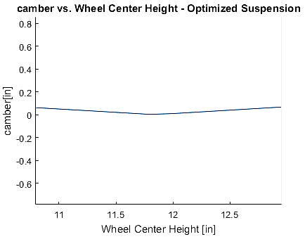
Figure 15 - Camber vs Ride Height Curve of optimized suspension

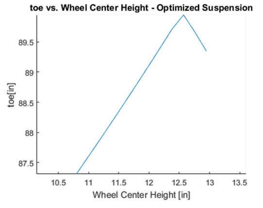
Figure 16 – Bump Steer vs Ride Height Curve of optimized suspension

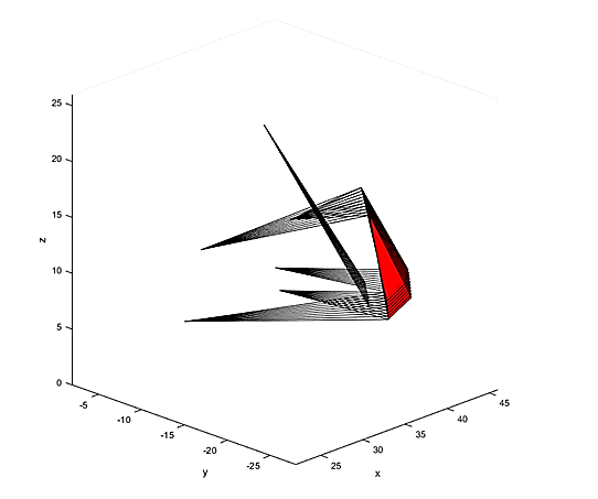
Figure 17 - Motion History of user specified motion range and steps

The baseline optimizer runs using FMINCON for 28 iterations with 168 function calls of the ‘solve_suspension’ function and converges to the following output:

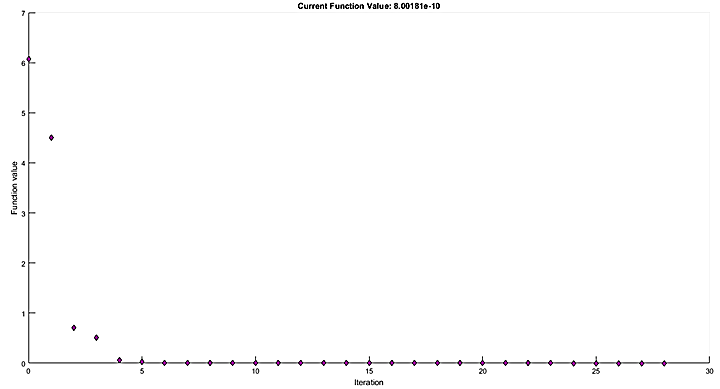
Figure 18 - Matlab FMINCON output of suspension optimization solver

Below a table presented for only the previous and new link lengths, while the rest of the outputs, such as the characteristic kinematic curves and the mass sizing optimization can be output by running the code again through Matlab.

Table 3 - Optimization Results

Original Link Lengths	Optimized Link Lengths
UCA, front: 11.8699 inch	UCA, front: 12.1275 inch

UCA, rear: 14.5911 inch
LCA, front: 13.5726 inch
LCA, rear: 17.1261 inch
Tierod: 15.9398 inch
UCA, rear: 15.1293 inch
LCA, front: 12.4872 inch
LCA, rear: 15.9100 inch
Tierod: 15.9249 inch

We can see that the optimizer does a good job of optimizing the camber gain. The resulting average camber gain is relatively linear which is a desirable characteristic and the average camber gain across the entire range of motion results in 1.956 degrees/inch (2.2% error in objective function). From the plots of the bump steer we can see that there is a increased non-linearity, which would typically be avoided in traditional design of a motorsports suspension, as well as an increased absolute bump steer across the entire jounce range.

Optimization Problem 2 – Optimized Camber Gain and Mass

Solution and Optimization

For the optimizer the following target kinematic curves for camber gain is used as the primary objective functions, in addition to the objective of mass minimization:

$camber\ gain = \frac{2^{\circ}}{\text{inch}} + min(overall\ mass)$

Due to the double objective function being minimized a weighted sum approach is used to give a single objective. The method of choosing the weights is done by normalizing the value of each individual objective against the initial value, and then summing them.

$Objective \equiv f\left( x \right) = w_{\text{mass}}*mass + w_{\text{camber}}*camber = \frac{1}{0.7315}*mass + \frac{1}{78.83}*camber$

The solver is the computed with the resulting camber and toe curves:

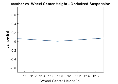
Figure 19 - Camber vs Ride Height Curve of optimized suspension

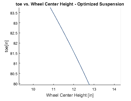
Figure 20 – Bump Steer vs Ride Height Curve of optimized suspension

The elasto-kinematic solver also runs for a total of three iterations with a resulting mass loss of 14.42% and a new structural sizing (which can be set as an output in the included Matlab code from the ‘calculate_optimal_sizing’ sub-function.

The baseline optimizer runs using FMINCON for 37 iterations with 256 function calls of the ‘solve_suspension’ function and converges to the following output:

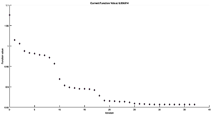
Figure 21 - Matlab FMINCON output of suspension optimization solver

Table 4 - Optimization Results

Original Link Lengths	Optimized Link Lengths
UCA, front: 11.8699 inch	UCA, front: 9.8699 inch

UCA, rear: 14.5911 inch
LCA, front: 13.5726 inch
LCA, rear: 17.1261 inch
Tierod: 15.9398 inch
UCA, rear: 13.3008 inch
LCA, front: 11.5726 inch
LCA, rear: 15.1261inch
Tierod: 13.9398 inch

It can be seen from these results that both camber gain and the mass is minimized. The same problem occurs with bump steer as for the single camber gain optimization case where the bump steer curve becomes more non-linear as well as increased in the absolute value. In general, it can be seen that the optimizer attempts to decrease all of the design variables (i.e. the length of each of the links) rather than focusing on the suspension metrics being optimized. This can be changed by modifying the weights of the various objectives of interest or doing a sweep of the weight in order to create a pareto frontier to see the relative entire multi-objective design space.

Optimization Problem 3 – Optimized Camber Gain and Mass

Solution and Optimization

For the optimizer the following target kinematic curves for camber gain is used as the primary objective functions, in addition to the objective of mass minimization:

$camber\ gain = \frac{2^{\circ}}{\text{inch}};\min\left( \text{overall\ mass} \right);bump\ steer = \frac{0^{\circ}}{\text{inch}}\$

$Objective \equiv f\left( x \right) = w_{\text{mass}}*mass + w_{\text{camber}}*camber + w_{\text{bumpSteer}}*BumpSteer\ = \frac{1}{0.7315}*mass + \frac{1}{78.83}*camber + \frac{1}{0.0363}*bumpsteer$

The solver is the computed with the resulting camber and toe curves:

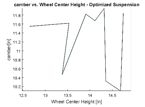
Figure 22 - Camber vs Ride Height Curve of optimized suspension

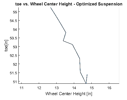
Figure 23 – Bump Steer vs Ride Height Curve of optimized suspension

The baseline optimizer runs using FMINCON for 3 iterations with 19 function calls of the ‘solve_suspension’ function and converges to the following output:

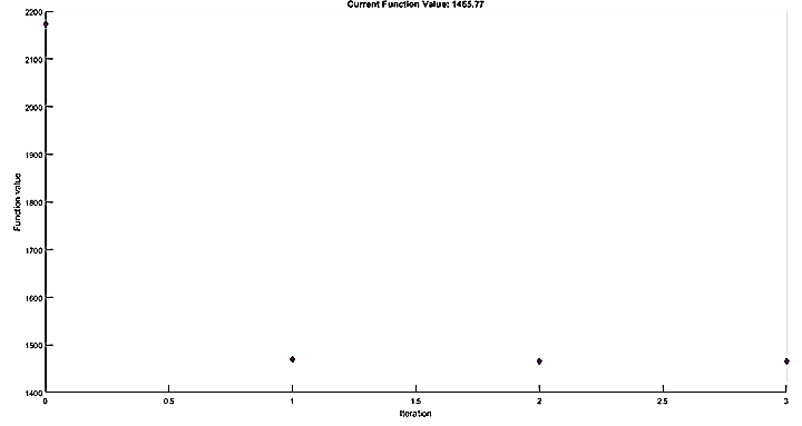
Figure 24 - Matlab FMINCON output of suspension optimization solver

Table 5 - Optimization Results

Original Link Lengths	Optimized Link Lengths
UCA, front: 11.8699 inch	UCA, front: 9.8699inch

UCA, rear: 14.5911 inch
LCA, front: 13.5726 inch
LCA, rear: 17.1261 inch
Tierod: 15.9398 inch
UCA, rear: 12.5911inch
LCA, front: 15.5726 inch
LCA, rear: 19.1261inch
Tierod: 17.9398 inch

Conclusion

In conclusion a framework was developed to model and analyze a Formula SAE style double a-arm independent suspension. This includes an iterative elasto-kinematic solver that allows for compliances under corner and braking loading throughout the range of motion. Finally, an optimal sizing sub-function is called under each solution step to minimize the weight of each of the six-independent links under yield and buckling criterion on the basis of the input material.

A MATLAB SQP based minimizer is used to solve the optimal solution for the distribution of link lengths and points. From the test case in which the camber is minimized by itself the desired camber gain curve is developed within 2% error. This though leads to non-linearities of bump steer curve leading to the necessity of a multi-objective minimization problem. When camber gain and mass are both minimized to their respective desired set points camber gain retains good accuracy to the 2 degrees per inch target (i.e. <5% error) and mass is reduced by about 14%. Finally, when all three objectives are minimized (camber gain, bump steer, and mass) there are large errors in both the camber and toe curves. This can be deduced to the large relative sensitivities of perturbances of each of the suspension points, as was calculated in the parametric study in Section 4.1.2. This leads to an ill-posed problem that has issues with minimizing into un-feasible local minima.

The resulting issues with the optimizer are related to the gradient descent method that is implemented in part with the SQP algorithm that is used. Due to the high non-linearity that was shown in the parametric study done to find the effects of suspension point perturbations to the resulting bumps steer curve a high degree of mismatch between the gradients for each of the design variables is present. Furthermore, a sign reversal is also present which can lead to instabilities in the resulting kinematic response curves which was shown in the last multiobjective optimization study (i.e. optimizing mass, camber gain, and bump steer simultaneously). Future work could be done in exploring various other optimization methods such as genetic algorithms and pattern search algorithms. The gradient descent method was originally chosen due to the continuous response of changes in the design variables to the resulting kinematic response curves, but the non-linearity was not explored soon enough to show that issues may arise.

Bibliography

“Formula SAE 2017-2018 Rules, SAE”, https://www.fsaeonline.com/page.aspx?pageid=e179e647-cb8c-4ab0-860c-ec69aae080a3
“Roark’s Formulas for Stress and Strain, 8th Edition”, Young Et. Al.
Milliken, D. L. (2003). Race car vehicle dynamics: problems, answers and experiments. Warrendale, PA: SAE International.
Smith, C. (1999). Tune to win. Redwood City, CA: Motorbooks International.
Dankowicz, H. (2010). Multibody Mechanics and Visualization
“Composites Design Binder”, Anthony Klepacki, 2017, Formula SAE Design Finals
http://static.competitionx.com/uploads/2010/09/rc-tuning-bumpsteer.jpg
http://www.liverc.com/news/special_features/13822-THE_SCIENCE_OF_SETUP%3A_Episode_5_-_Camber_and_Camber_Gain_%5BVIDEO%5D/
“Illini Motorsports Website”,Motorsports.illinois.edu
‘SAE J760: Vehicle Dynamics Terminology’, SAE International,1996, Revised 2008